


Decommissioned Optimization, (Pseudo-)Vectoriozation, and Parallelization for SR8000
Tuning and Optimization Manuals, Courses and Lectures
Advanced techniques of optimization
- Optimization, (Pseudo-)Vectorization, and Parallelization on the Hitachi SR8000-F1
- Basic Optimization Strategies for CFD-Codes
- A Supplement to the Hitachi SR8000 Tuning Manual, written by the High Performance Computing Group of LRZ, Postscript.
- written by the High Performance Computing Group of Regionales Rechenzentrum Erlangen, PDF.
High Precision Clocks and Cycle Counters
Cycle Counters: $SCETCYC
This routine returns the number of machine cycles as an INTEGER (KIND=8) value.
Usage:INTEGER (KIND=8) CYCLES1,CYCLES2 CALL $SGETCYC(CYCLES1) ... code to be measured CALL $SGETCYC(CYCLES2) write(6,*) 'Cycles used ', CYCLES2-CYCLES1
Timing Routines
Service routines available in Fortran:
XCLOCKreturns elapsed or CPU timesPCLOCKmeasures the CPU time required for parallel processing. The routine calculates the maximum, minimum and average values for all the threads.real*8 p(4)call pclock(p,3)... code to be measuredcall pclock(p,8)p(1): The maximum CPU time of all of the threads from the PCLOCK(p,3)p(2): The minimum CPU time of all of the threads from the PCLOCK(p,3)p(3): The average CPU time of all of the threads from the PCLOCK(p,3)p(4): The same value as p(3)
The following routines are contained in liblrz
DWALLTIMEreturns the elapsed wallclock time; uses mk_gettimeofday.double dwalltime()DOUBLE PRECISION FUNCTION DWALLTIME()DCPUTIMEreturns the used CPU time; uses getrusage.double dcputime()DOUBLE PRECISION FUNCTION DCPUTIME()SECOND/DSECONDreturns the used CPU time; uses XCLOCK.REAL*4 FUNCTION SECOND()REAL*8 FUNCTION DSECOND()SECONDR/DSECONDRreturns the elapsed wallclock time; uses XCLOCKREAL*4 FUNCTION SECONDR()REAL*4 FUNCTION DSECONDR()TREMAINreturns the remaining CPU time; uses XCLOCK.DOUBLE PRECISION FUNCTION TREMAIN()
Stopwatch
StopWatch is a Fortran 90 module for portable, easy-to-use measurement of execution time. It supports four clocks -- wall clock, CPU clock, user CPU clock and system CPU clock -- and returns all times in seconds. It provides a simple means of determining which clocks are available, and the precision of those clocks. StopWatch is used by instrumenting your code with subroutine calls that mimic the operation of a stop watch. StopWatch supports multiple watches, and provides the concept of watch groups to allow functions to operate on multiple watches simultaneously.Location of libraries and modules: /usr/local/lib/stopwatchDocumentation: user's guide (html), user's guide (postscript), man pages
Hardware Performance Counters
NQS Output
- A very easy way to get information about the performance is to look into the NQS output file. At the end of a job the following information is output:
"------------------------------  job end log  -----------------------------------"
"executed user id                     = $QSUB_UID"
"executed group id                    = $QSUB_GID"
"executed group name                  = $QSUB_GROUP"
"account number                       = $SHOW_ACCT"
"request id                           = $QSUB_REQID"
"submitted queue name                 = $QSUB_QNAME"
"request end status                   = $QSUB_STATUS"
"request exit code                    = $QSUB_REXIT"
"user cpu time                        = $QSUB_UTIME (sec.nanosec)"
"system cpu time                      = $QSUB_STIME (sec.nanosec)"
"request existed time                 = $QSUB_ETIME (sec)"
"submitted time                       = $QSUB_SUBT"
"number of forked processes           = $QSUB_NFPRC"
"request priority                     = $QSUB_RPRI"
"queue priority                       = $QSUB_QPRI"
"submitted host name                  = $QSUB_HOST"
"submitted user name                  = $QSUB_LOGNAME"
"request start time                   = $QSUB_RST"
"request end time                     = $QSUB_RFT"
"executed host name                   = $QSUB_EXECHOST"
"integrated memory size               = $QSUB_PGMEM (kilobytes)"
"maximum rss size                     = $QSUB_MAXRSS (kilobytes)"
"number of read or wrote blocks       = $QSUB_RWBLOCK (blocks)"
"number of read or wrote chars        = $QSUB_RWBYTE (bytes)"
"number of shared nodes               = $QSUB_asnoODE"
"shared nodes time                    = $QSUB_SNODETIME (sec.nanosec)"
"number of exclusive nodes            = $QSUB_AENODE"
"exclusive nodes time                 = $QSUB_ENODETIME (sec.nanosec)"
"number of threads                    = $QSUB_THREADS"
"number of element parallel processes = $QSUB_EPNPRC"
"total computing time of"
"      element parallel processes     = $QSUB_EPTIME (sec.nanosec)"
"scalar computing time of"
"      element parallel processes     = $QSUB_EPSCATIME (sec.nanosec)"
"parallel computing time of"
"      element parallel processes     = $QSUB_EPPARTIME (sec.nanosec)"
"number of processors per"
"      element parallel process       = $QSUB_EPNUM"
"scalar barrier waiting time of"
"      element parallel processes     = $QSUB_EPSCABWTIME (sec.nanosec)"
"parallel barrier waiting time of"
"      element parallel processes     = $QSUB_EPBWTIME (sec.nanosec)"
"used ES size                         = $QSUB_ESSIZE (megabytes)"
"number of instruction TLB miss       = $QSUB_ITLBMISS"
"number of data TLB miss              = $QSUB_DTLBMISS"
"number of instruction cache miss     = $QSUB_ICACHEMISS"
"number of data cache miss            = $QSUB_DCACHEMISS"
"number of memory access instructions = $QSUB_AUCOMPL"
"number of all instructions           = $QSUB_INSCOMPL"
"number of floating point"
"                     instructions    = $QSUB_FPCOMPL"
"floating point instructions per sec. = $QSUB_FPCOUNTER (FLOPS)"
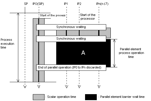
Figure 1: shows the operation of the parallel element program.
The following explains in detail the environment variables which are used in the output
QSUB_EPSCATIME
Indicates the value that the parallel element program shown in Figure 4-3 outputs by adding the scalar operation times for all processes within one request of NQS.
- QSUB_EPPARTIME
Indicates the value (vertical length of section A) output by the parallel element program in Figure 1. The program obtains this value by adding the parallel element process operation times for all processes within one request of NQS.
- QSUB_EPSCBTIME
Indicates the value output by the parallel element program in Figure 1 The program obtained this value by adding up the barrier wait times generated on SIP for all processes within one NQS request. (Figure 1 omits the barrier wait time on SIP.)
- QSUB_EPBWTIME
Indicates the value (total of IP1 to IPn) output by the parallel element program in Figure 1 The program obtains this value by adding the barrier wait times generated on IP for all processes within one NQS request.
- QSUB_EPTIME
Indicates the value output by the parallel element program shown in Figure 4-3. The program obtains this value by adding the following values for all processes within one NQS request: the scalar operation time and the total (area of section A) of the parallel element process operation times for all IPs.
Parallel level : You can use the ratio of QSUB_EPSCATIME to QSUB_EPPARTIME as the parallel ratio of the parallel element program.
- QSUB_SNODETIME and QSUB_ENODETIME
Indicates the product obtained by multiplying the following two items together: node numbers ( QSUB_ASNODE or QSUB_ASENODE) specified by qsub -N of NQS or #@$-N of the script and the time from successful node reservation to node reservation release.
QSUB_SNODETIME
indicates the value for the nodes having the shared attribute, while QSUB_ENODETIME indicates the value for the nodes having the exclusive attribute. The next Figure shows these values as the product obtained by multiplying the elapsed time between A and B by the node numbers.
Time during which NQS assumes the node allocation status:
QSUB_MAXRSS
Indicates the physical memory value of the process that most frequently uses the physical memory within the NQS request. Example: QSUB_MAXRSS is 200 megabytes for these processes: a process that uses a maximum of 100 megabytes of physical memory and a process that uses a maximum of 200 megabytes of physical memory.
- QSUB_PGMEM
Indicates the total of the average real memory usage of the processes within the NQS requests. The average real memory usage is obtained by dividing the time integral of the physical memory usage by the integrated time.
Example: QSUB_PGMEM is 300 megabytes for these processes: a process whose average real memory usage is 100 megabytes and a process whose average real memory usage is 200 megabytes.
- QSUB_ESSIZE
Indicates the total peak value of the extended storage usage the processes within the NQS requests.
Example: QSUB_ESSIZE is 300 megabytes for these processes: a process that uses a maximum of 100 megabytes of extended storage and a process that uses a maximum of 200 megabytes of extended storage.
- QSUB_THREADS
Indicates the total of the threads of the processes within the NQS-generated requests. For those programs whose threads continue growing, this value is cumulative.
- QSUB_EPNPRC
Indicates the total number of processes that execute parallel element programs in each process within the NQS-generated requests. This value is an internal number of QSUB_NFPRC. If ten processes were executed and eight of them will execute parallel element programs, then QSUB_NFPRC is 10 and QSUB_ENPRC is 8.
Hardware Counters in the NQS output:
- Any of the environment variables listed below indicates the total value for all the processes included in the NQS requests. The following also gives the meaning of each environment variable :
- QSUB_ICACHEMISS: Number of times that an instruction cache error occurs
- QSUB_DCACHEMISS: Number of times that a data cache error occurs
- QSUB_ITLBMISS: Number of times that an instruction TLB error occurs
- QSUB_DTLB_MISS: Number of times that a data TLB error occurs
- QSUB_AUCOMPL: Number of times that the memory access instruction is executed
- QSUB_INSCOMPL: Total number of times that all instructions are executed
- QSUB_FPCOPL: Number of times that floating-point arithmetic is executed
- QSUB_FPCOUNTER: Number of times that floating-point arithmetic is executed for one second per IP, based on the user CPU time.
- For a parallel element job, you can obtain the number of times that floating-point arithmetic is executed per node, by multiplying the QSUB_FPCOUNTER value by the number of parallel element process parallels (QSUB_EPNUM).
- For a scalar job, uses, as is, the number of times that the floating-point arithmetic is executed per IP.
- For full details see: OSCNQS System Administrator's Guide and Reference.
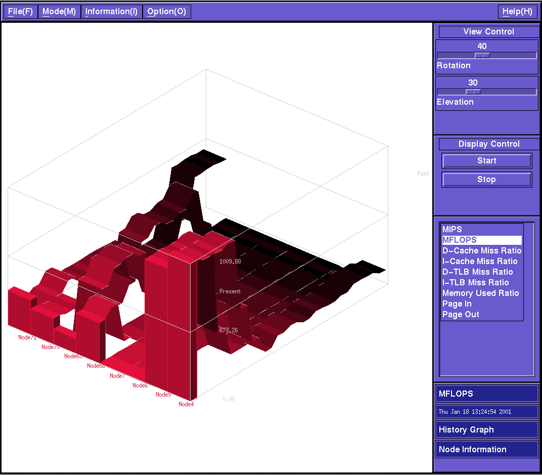
Real Time Monitor
- For detail see: Realtime Monitor Description and User's Guide.
- Currently the Real Time Monitor can only be used in batchmode (writing a logfile) or interactively for the partition IAPAR.
Running Interactively
- Start the server with the command: PMSERVER
- Select the parameters you want, e.g. the sampling interval
- Start the Topology or History Graph
- Select the appropriate data to be displayed e.g. MFLOPS.
- (in the case the server has been already started by another user, use the PMHISTORY or PMTOPOLOGY command to start these displays)
pmexec
Usage: pmexec [-g <process number> ] <command> [arg...]
pmexec -p [-i <interval>] [-g <process number>] [<command> [arg...]]
pmexec -a [-i <interval>]
pmexec -G [-i <interval>]
-g: Monitoring process number(0-9).[default:0]
-p: Displays performance data of monitored processes.
-a: Displays performance data of all processes.
-i: Displays performance with specified interval in seconds.
-G: Displays graphical cpu usage.
The following values are displayed(local node processes only):
usr(s) User cpu time(seconds).
(us) User cpu time(micro seconds).
sys(s) System cpu time(seconds).
(us) System cpu time(micro seconds).
usage CPU usage(%) [(usr+sys)/etime].
inst Number of instructions.
CPI Clocks Per Instructions.
LD/ST Number of Load and Store instructions.
ITLB Number of Instruction-TLB miss.
DTLB Number of Data-TLB miss.
Icache Number of Instruction-Cache miss.
Dcache Number of Data-Cache miss.
FU Number of Floating instructions.
fault Number of page faults.
zero Number of zero pages(page allocations).
react Number of reactivations(pageout cancels).
pagein Number of pageins.
COW Number of Copy-On-Write.
nswap Number of swapouts.
syscall Number of system-calls.
align Number of page alignment fault
Automatic Instrumentation with -Xparmonitor or -Xfuncmonitor
InstrumentationTo instrument the code, compile with
if you are interested in parallel perfomance or with
- f90 -model=F1 -opt=ss -Xparmonitor ...
if you are interested just in the performance of routines. This adds instrumentation around each parallel section of the subroutine. Several sets of data will be produced for each routine: one set for each parallel region of the code and one set for all the serial sections combined. (Remark) Even if the code is not being compiled with COMPAS enabled, -Xparmonitor is suitable.
- f90 -model=F1 -opt=ss -Xfuncmonitor ...
f90 -model=F1 -opt=ss -noparallel -Xfuncmonitor ...Linking
This links to the performance monitor library. The monitor library makes some calls to other libraries, and the easiest way to ensure that all libraries are present is to use the -parallel option.
- Link with f90 [-32|-64] -parallel ... -lpl for COMPAS
- Link with f90 [-32|-64] -noparallel ... -lpl -lcompas -lpthreads -lc_r for non-COMPAS programs
Set an environment variable to select the type of output file that is produced
export APDEV_OUTPUT_TYPE=TEXT (in sh/ksh)The value TEXT produces a human readable output file, CSV produces and comma separated variable file suitable for processing by tools such are spreadsheets and BOTH produces both files. The default value if the variable is not set is TEXT. Use CSV to be able to process data by my tool mentioned in
export APDEV_OUTPUT_TYPE=CSV (in sh/ksh)
export APDEV_OUTPUT_TYPE=BOTH (in sh/ksh)Run the job
After completion, one file per MPI process will be written. The file name will be of the form: executable_name_process_id_node_number.[csv|txt]
Evaluate the data
The Perl script mon.pl (installed in /usr/local/bin) to extract some useful data from the CSV files. Run with mon.pl -f file.csv to get Mflops related data and mon.pl -t file.csv to get time related data. This script was written for personal use and as an example of how to extract data from the hardware monitor files. It is not a supported Hitachi product. Be also aware that the parallel part of routine which are not instrumented (e.g., The BLAS library) could not be counted correctly.
Automatic instrumentation with -pmfunc, -pmpar and pmpr
The same measurements as for -Xfuncmonitor and -Xparmonitor are performed, if the code is compilled with -pmfunc and/or -pmpar, but the method of output is a bit different.Instrumentation
Compile and link with:
FORTRAN compiler supposes to be specified at least -O4 optimization option (level 4) when -pmfunc or -pmpar option is specified. And the C compiler supposes to be specified at least -O3 optimization option (level 3) when -pmfunc or -pmpar option is specified.
- f90 -model=F1 -opt=ss -pmfunc -pmpar ...
Performance monitoring information file:
A performance monitoring information file is created by the performance monitoring library when an application program runs. For example, if the program was executed with the following conditions, the name of the performance monitoring information file is pm_PROGRAM_Jan02_0304_node005_6
1. Load module name : PROGRAM
2. Execution start time: January 2nd, at 4 minutes past 3.
3. Node no : 5
4. Process no 6Output the information
The pmpr command inputs this performance monitoring information file and displays various types of performance monitoring information (see pmpr(1)), e.g.:
- pmpr -ex -full pm_PROGRAM_Jan02_0304_node005_6
this will give a full output with explanations. See output file for details.
- pmpr -c -full pm_PROGRAM_Jan02_0304_node005_6
this will output a comma seperated list for the use with spread sheets.
Details of the performance monitoring information
Beware: If a routine calls non-instrumented subroutines (e. g. libraries), the MFlops/timings of the latter are folded into the calling routines measurement!Checking the contents of a performance monitoring information files enables you to obtain various types of performance monitoring information: such as the CPU time (the period required by the CPU to execute a program), the number of executed instructions, and the number of floating-point operations. Details of the performance monitoring information are as follows:
Performance monitoring information for a process:
Performance monitoring information in units of functions or procedures:
- Program execution starting date and time
- Node no
- Process no
- Load module name
- Input/Output count
- Input/Output quantity
- CPU time
- LoaD/STore instructions count
- execution instructions count
- Number of floating-point operations
- MIPS
- MFLOPS
- Number of data cache misses
Performance monitoring information in units of element.
- Function or procedure name
- Source file name
- Starting-line number
- Number of executions
- CPU time
- LoaD/STore instructions count
- execution instructions count
- Number of floating-point operations
- MIPS
- MFLOPS
- Number of data cache misses
- Execution rate (time basis)
- Element parallelizing rate (CPU time and floating-point operations)
- Types of information are the same as the performance monitoring information when the units are functions or procedures.
PCL: Performance Counter Library
(currently only available for non-COMPAS programs)Introduction
To optimize program performance, it is important to know where the bottlenecks are located. One means to identify bottlenecks in the program code is through the use of hardware counters. For example, such hardware counters can count floating point instructions, cache misses, TLB misses, etc. It is important to use hardware counters and not software counters to keep the overhead to a minimum and thus reduce the disturbing impact on the user program. This is especially important for parallel programs.
Currently, the low level interface to the SR8000 hardware counters is not yet published. However, there is a platform-independent high level interface called "Performance Counter library", or short PCL, of Forschungszentrum Juelich GmbH, which has been ported to the Hitachi SR8000 by LRZ staff and which hides all the gory details of the low level interface. These routines can and should be used by SR8000 users to instrument their programs.
PCL
PCL was developed by Rudolf Berrendorf and Heinz Ziegler at the Central Institute for Applied Mathematics (ZAM) at the Research Centre Juelich, Germany. It is a library which can be linked with your code and which provides a high level, platform-independent interface to hardware performance counters. These high level library calls can be used to instrument your code and yet keep it portable. PCL also allows nested calls - up to a certain, pre-compiled limit, which is currently set to 16 nesting levels. For more information, please have a look at the PostScript documentation.
On the -SR8000 the LRZ installed the latest pre-release of PCL, version 2.0. The library resides in /usr/local/lib/libpcl32s.a and can be linked with -lpcl32s. The include files pcl.h for C code and pclh.f for FORTRAN code can be found in /usr/local/include.
Only the following hardware counters (PCL_EVENT) are currently supported on the SR8000:
PCL_L1DCACHE_MISS (Data Cache misses)
PCL_L1ICACHE_MISS (Instruction Cache misses)
PCL_DTLB_MISS (Data Translation Lookup Buffer misses)
PCL_ITLB_MISS (Instruction Translation Lookup Buffer misses)
PCL_CYCLES (Cycles)
PCL_ELAPSED_CYCLES (Elapsed Cycles)
PCL_FP_INSTR (Floating Point Instructions)
PCL_LOADSTORE_INSTR (Number of Load-Store Instructions)
PCL_INSTR (All Instructions)
PCL_MFLOPS (MFlops)
PCL_IPC (Instructions per Cycle)
PCL_L1DCACHE_MISSRATE (Data Cache Miss Rate)
PCL_MEM_FP_RATIO (Memory Instructions to Floating Point Instructions Ratio)The small example program ptest.c illustrates how a program can be instrumented. Please compile and link it like this
cc -o pcltest -I/usr/local/include -L/usr/local/lib ptest.c -lpcl32sSample output for this program is provided here:
FLOPs in iteration 0: 1
FLOPs in iteration 1: 101
FLOPs in iteration 2: 201
FLOPs in iteration 3: 301
Total FLOP count: 604We would like to point out that the total FLOP count in this example was not computed by adding the individual loop contributions, but through the use of nested counters!
AutoPCL
To make life a bit easier for our users, LRZ also installed autoPCL, which was programmed by Touati Sid Ahmed Ali of INRIA, France. AutoPCL is a tool that automatically inserts calls to PCL in your FORTRAN source. Unfortunately, autopcl permits only the counting of one event at a time in a Fortran code section and is therefore only of limited practical usability. However, it can be used as a first approach to PCL and the resulting instrumented code can serve as a template for your own, manual instrumentation.
AutoPCL can be called as follows:
autopcl -i fortest -p PCL_FP_INSTR -m PCL_MODE_USER -b7 -e9
The options have the following meaning:
-i <input fortran file name without .f extension>
-p <type of counter, here floating point instructions, cf. table of supported counters>
-m <mode. Must be PCL_MODE_USER for now>
-b<line number in original fortran file where to start monitoring>
-e<line number in original fortran file where to stop monitoring>The example program fortest.f is transformed into instrumented code, which can be found here ipcl.f.
LRZ-Extensions
The LRZ is currently working on a few extensions for automatic instrumentation of user programs. Stay tuned for more information.
PMCINFO: Low Level Hardware Performance Counters
(These counters are available for COMPAS and non-COMPAS programs)The routines are contained in liblrz
PMCINFO_S(COUNTERS)
returns the Hardware counters for a serial program
I